Statistic annotations with python

“Look what they need to mimic a fraction of our power.”

When we plot graphs comparing quantitative metrics between groups, we often need to add statistical annotations to the plot to denote differences between groups. While programs such as GraphPad Prism and SPSS has built-in tools to add statistical annotations, they lack flexibility and customisability.

This post will introduce programmatic statistical annotations using Python via the statannotations package, using the iris dataset

Prerequisite

• Python >= 3.8
• matplotlib
• seaborn
• statannotations

Installation

pip install statannotations

OR

conda install -c conda-forge statannotations

Usage

1. Import packages and load data

    import matplotlib.pyplot as plt
    import seaborn as sns
    from statannotations.Annotator import Annotator #this is statannotations
    from itertools import pairwise, permutations, combinations
    df = sns.load_dataset("iris")
   

2. Set the x and y variables, order and combinations of comparisons

    x = "species"
    y = "petal_width"
    order = ['setosa', 'versicolor', 'virginica']
    combo = [(x, y) for x, y in combinations(order, 2)]
   

   In this case we want to do a pair-wise comparison between setosa, versicolor and virginica

3. Initialise the plot

    ax = sns.boxplot(data=df, x=x, y=y, hue=x, order=order, hue_order=order)
   

4. Initalise the annotator object

   The annotator takes your plot object, comparison comaprisons, dataset, x and y variables, and order

    annot = Annotator(ax, combo, data=df, x=x, y=y, order=order)
   

5. Configure and apply the test statistic

    annot.configure(test='Mann-Whitney', comparisons_correction="Bonferroni", text_format='star', loc='outside', verbose=2)
   
    annot.apply_test()
   

6. Annotate the plot

    ax, test_results = annot.annotate()
    plt.show()
   

   The loc parameter controls how the annotations are placed, outside means they are placed outside the plot, while inside means they are placed inside the plot

   Outside (loc='outside')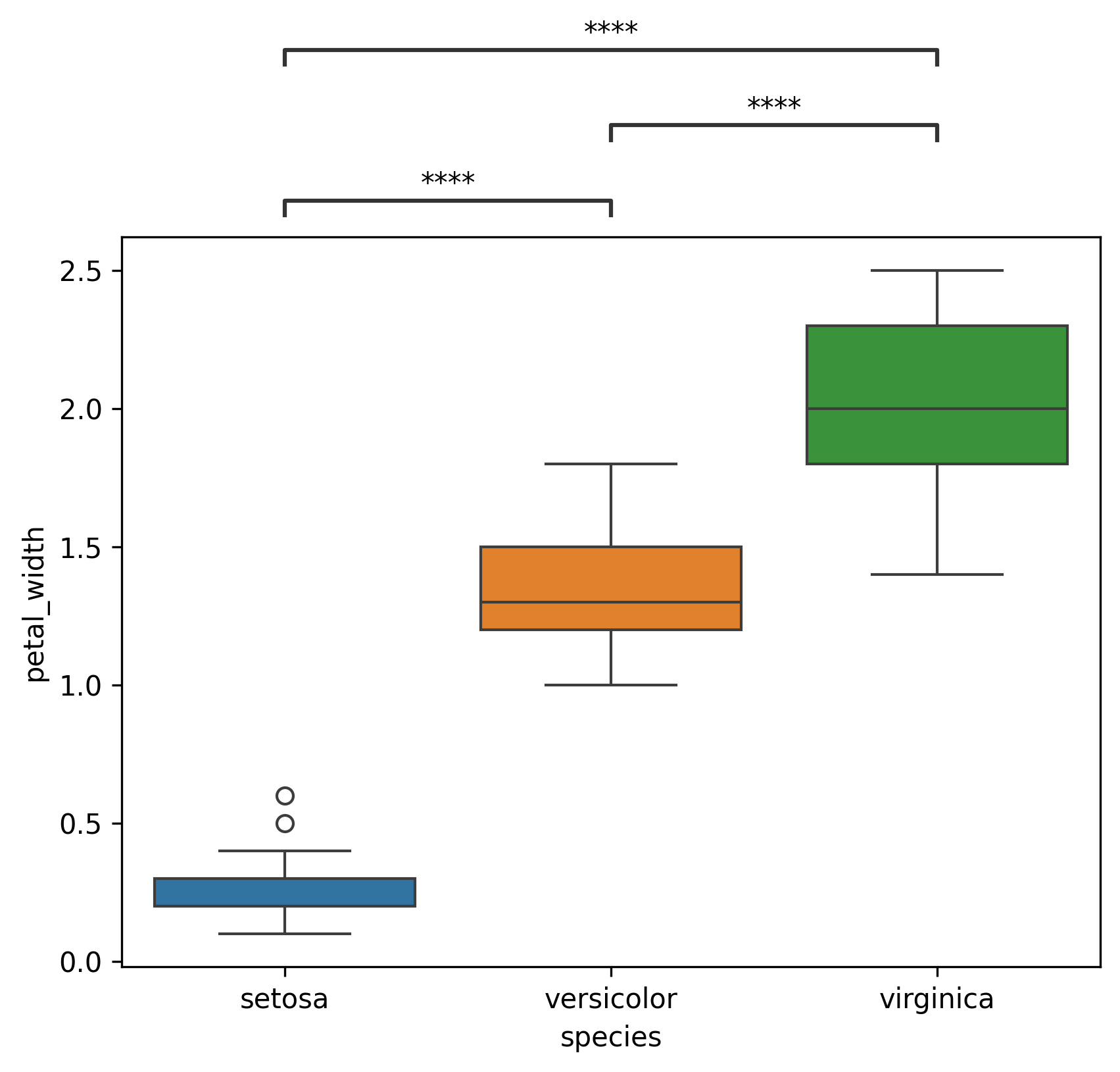

   Inside (loc='inside')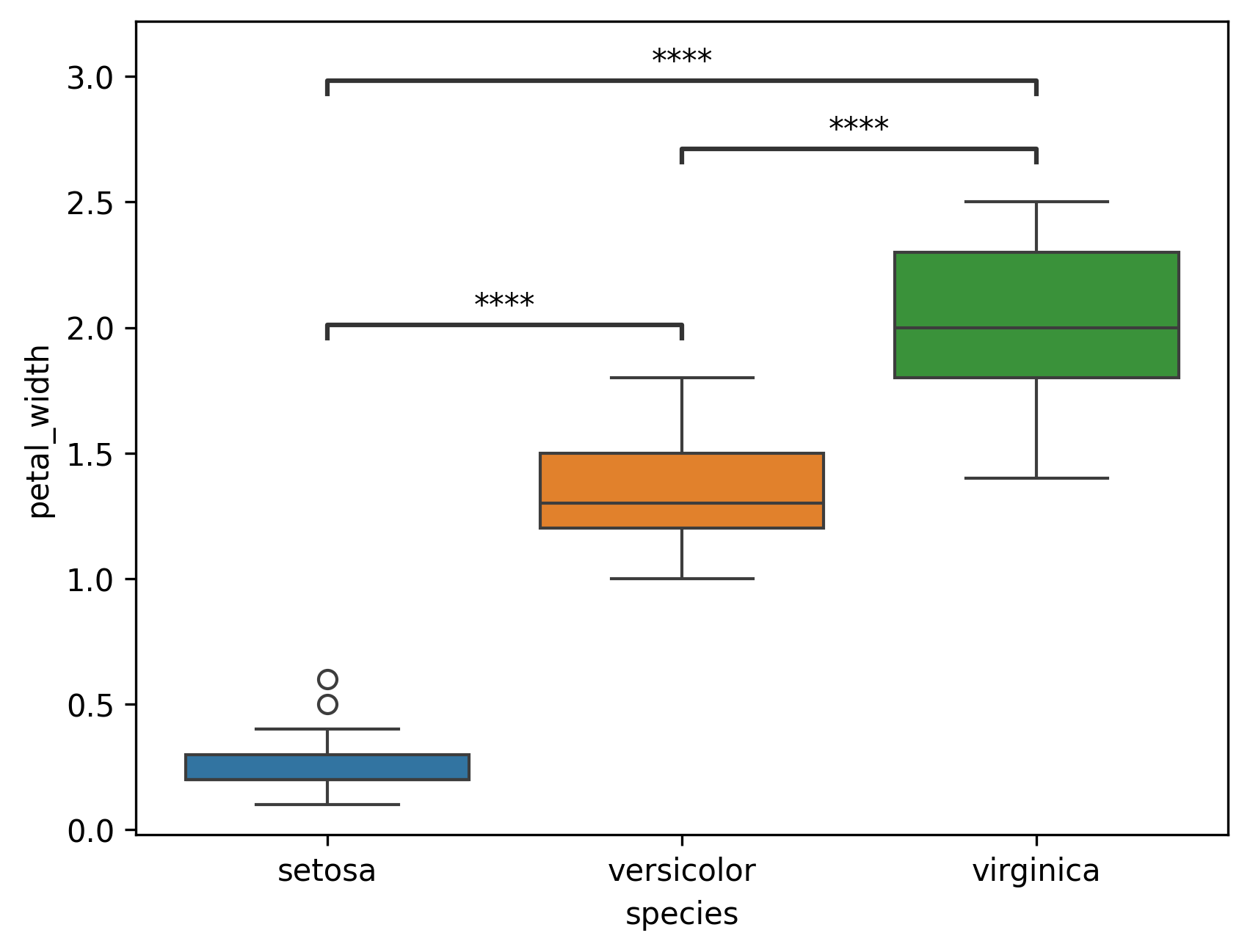

7. Alternatively, the plotting can be done using a config dictionary

   Set a config dictionary

    plotting = {
    "data": df,
    "x": x,
    "y": y,
    "hue": x,
    "hue_order": order,
    "order": order
    }
   

   Plotting

    ax = sns.boxplot(**plotting)
   

   Configure annotation + multiple tests

    annot.new_plot(ax, **plotting)
    annot.configure(comparisons_correction="Bonferroni", verbose=2)
   

   Apply test and annotate (You can daisy-chain the functions)

    test_results = annot.apply_test().annotate()
   

Reference

1. https://github.com/trevismd/statannotations

back