Visualisation of protein domains architecture

Representing protein domain architecture is often used in research, especially when investigating unknown sequences.

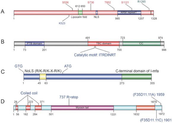
They usually look like this.

However, the DOG1.0 appears to deprecated. IBS2.0 is an now available plotter for biological sequences, not just protein domains.

Apart from manually drawing it by hand, you could programmatically and dynamically make these plots. However, currently available tools is limited to the R programming language.

drawProteins and seqvisr are two of such tools. I will be covering drawProteins and how to customise the plots by using the BoNT/A (accession: Q7B8V4) from C. botulinum as an example.

Prerequisite

• R (>=4.3.3)

testing on older versions worked without issues, but is not guaranteed

Installation

if (!require("BiocManager", quietly = TRUE))
    install.packages("BiocManager")

BiocManager::install("drawProteins")

Usage

1. Load the packages

    library(drawProteins)
    library(ggplot2) #optional
   

2. Load in the data.

   By default, drawProteins can load uniprot to load the information. You will able to directly use the information from the annotation

    json_dat <- get_features("Q7B8V4")
    df_dat <- feature_to_dataframe(json_dat)
   

   alternatively, load it in one go with

    df_dat <- feature_to_dataframe(getfeatures("Q7B8V4"))
   

3. Intialise the ggplot canvas

    p <- draw_canvas(df_dat)
   

4. Plot the chains and domains

    p <- draw_chains(x, df_dat)
    p <- draw_domains(x, df_dat)
   

5. Optional: Modify the plot the remove background and change the theme, along with setting the font face. You will need ggplot2 imported

    p + theme_bw(base_size = 20, base_family = "Times New Roman" )
    theme(panel.grid.minor=element_blank(), 
          panel.grid.major=element_blank()) +
    theme(axis.ticks = element_blank(), 
          axis.text.y = element_blank()) +
    theme(panel.border = element_blank()) +
    theme(legend.title = element_text(size = 20))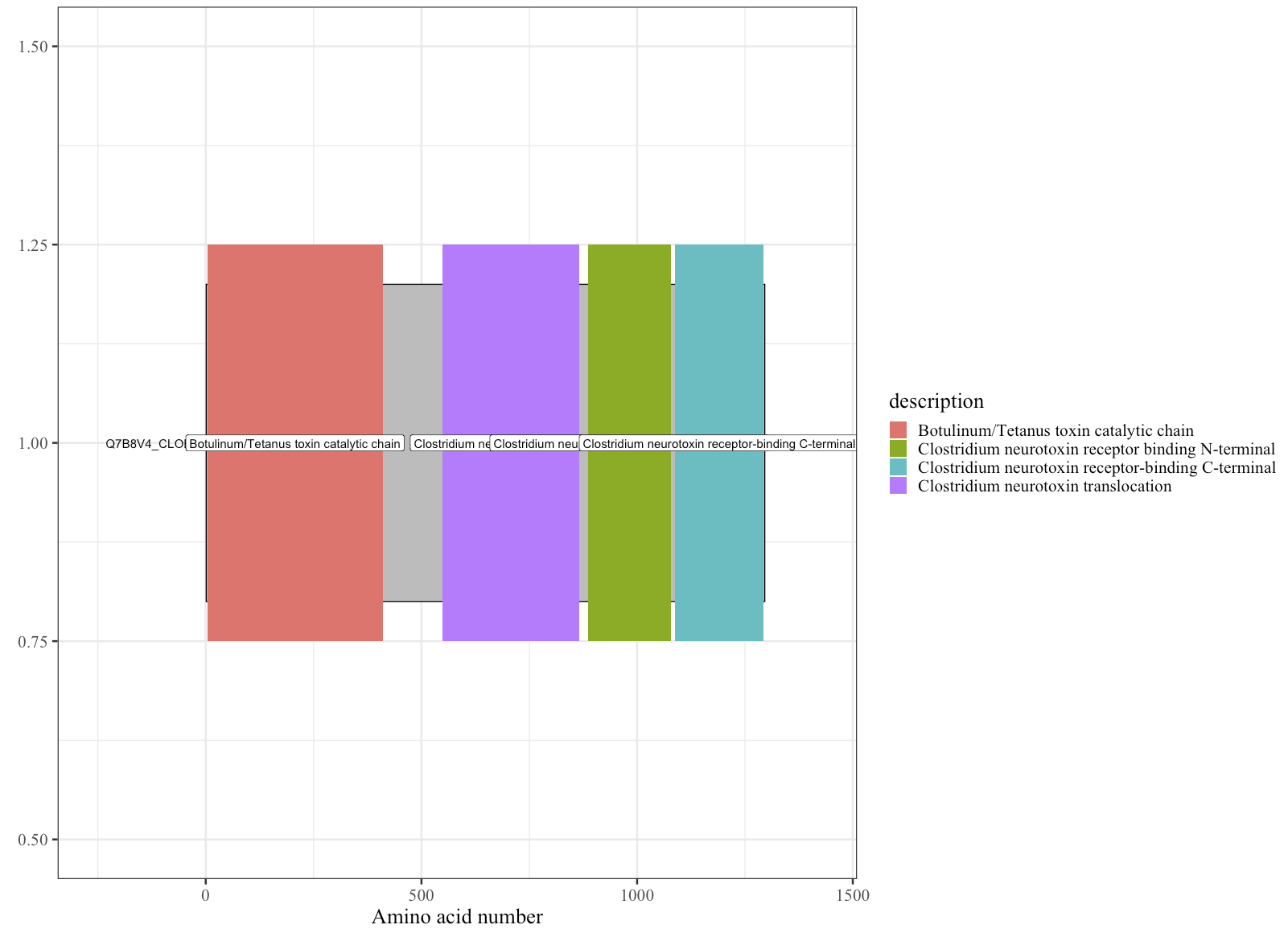
   

   

   Note: the documentation is lacking, and doesn’t cover other aspects of modfiying the plot

   Remove the description on the domains by adding label_domains = FALSE to draw_domains

    p <- draw_domains(x, df_dat, label_domains = FALSE)
   

   Change the legend title and key size

    p <- p + guides(fill=guide_legend(title="Features", keywidth = unit(2, 'cm')))
   

   

   Set a colour palaette for your domains, using the okabe colour blind friendly set as example

    okabe <- c("#D55E00", "#CC79A7", "#E69F00", "#009E73", "#0072B2")
   
    p <- p + scale_fill_manual(values = okabe)
   

   

   Note that the accession id on the left side is not Times new roman. This is because the draw_chains calls ggplot to annotate the file beforehand, it escapes the theme_bw(base_family=font) override command. We want define a new function, say draw_chains_times as

    draw_chains_times <- function (p, data = data, outline = "black", fill = "grey", label_chains = TRUE, 
                               labels = data[data$type == "CHAIN", ]$entryName, size = 0.5, 
                               label_size = 4) 
    {
    begin = end = NULL
    p <- p + geom_rect(data = data[data$type == "CHAIN", 
    ], mapping = aes(xmin = begin, xmax = end, ymin = order - 
                                  0.2, ymax = order + 0.2), colour = outline, fill = fill, 
    size = size)
    if (label_chains == TRUE) {
        p <- p + annotate("text", x = -10, y = data[data$type == "CHAIN", ]$order, 
                                   label = labels, 
                                   hjust = 1, 
                                   size = label_size, 
                                   family = "Times")
    } 
    return(p)
    }
   

   Note: if you have already imported ggplot2, do not add ggplot2:: in front of geom_rect and annotate in the custom function

   Now intsead of calling draw_chains, call draw_chains_times or any other name you have defined in this custom function.

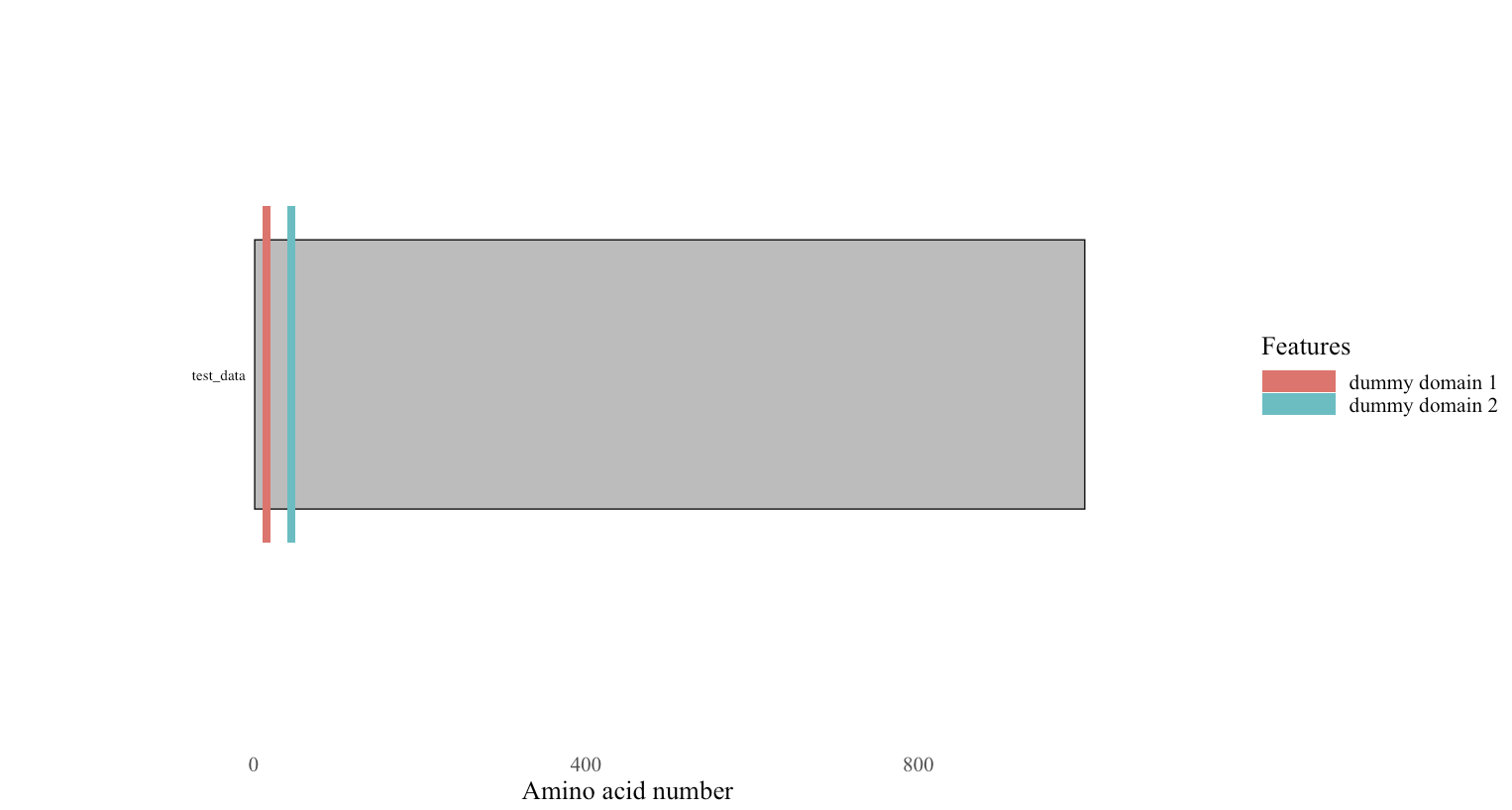
6. You can plot custom proteins in case Uniprot annotation is not up to your taste/not available.

   This is done by injecting a dataframe in this format:

   rowname	type	description	begin	end	length	accession	entryName	taxid	order
   1	CHAIN	dummy	1	1000	1000	test_dummy	test_data	1	1
   2	DOMAIN	dummy domain 1	10	20	10	dummy domain	dummy domain	1	1
   3	DOMAIN	dummy domain 2	40	50	10	dummy domain	dummy domain	1	1

   this represents a protein of size 1000, with two domains at 10-20 aa and 40-50 aa. I have placed taxid as 1 as placeholder

   Assuming your data is in a file called dummy_data.txt in the same current working directory.

   library(data.table)
   df_dat <- data.frame(fread("./dummy_data.txt"), row.names = 1)
   

   row.names = 1 means the first column is the row names.

   Now plot as you would in the previous example.

   

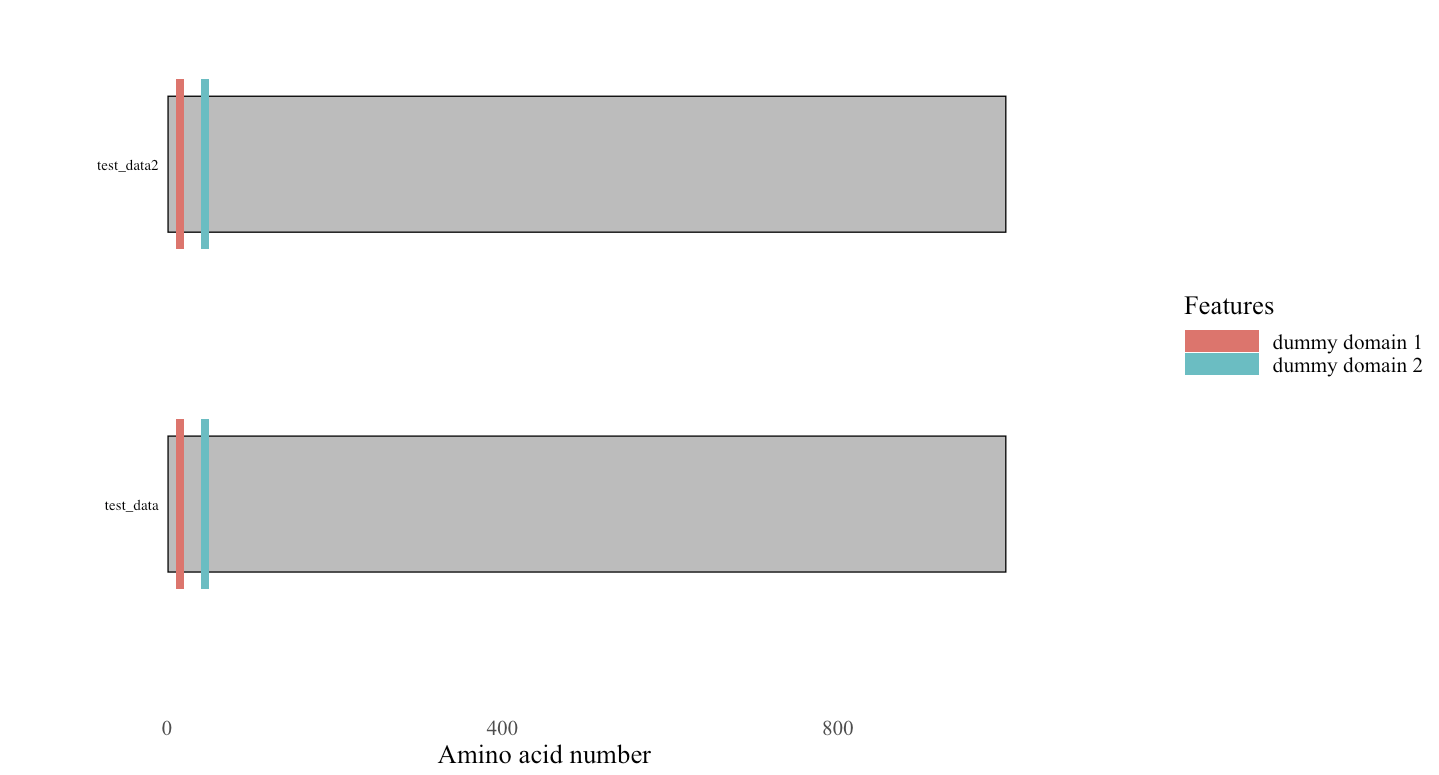
   This can be extended to plot multiple proteins.

   rowname	type	description	begin	end	length	accession	entryName	taxid	order
   1	CHAIN	dummy	1	1000	1000	test_dummy	test_data	1	1
   2	DOMAIN	dummy domain 1	10	20	10	dummy domain	dummy domain	1	1
   3	DOMAIN	dummy domain 2	40	50	10	dummy domain	dummy domain	1	1
   4	CHAIN	dummy	1	1000	1000	test_dummy	test_data2	1	2
   5	DOMAIN	dummy domain 1	10	20	10	dummy domain	dummy domain	1	2
   6	DOMAIN	dummy domain 2	40	50	10	dummy domain	dummy domain	1	2

   By adding to the order row, you can plot multiple proteins.

   Note: plots are made from bottom up. Keep that in mind.

   

Reference

1. https://f1000research.com/articles/7-1105/v1

back