Visualisation of phylogenetic tree using ggtree

“But the difficulty is not nearly so great as it at first appears: all this beautiful work can be shown, I think, to follow from a few very simple instincts” - Charles Darwin, 24 November 1859, On the Origin of Species

Following up from inferrence of phylogenetic tree from this tutorial, this tutorial will show how the tree can be visualised using R using ggtree and ggtreeExtra.

Prerequisite

• R
• ggplot2
• ggtree
• ggtreeExtra
• phangorn
• treeio
• ggnewscale

Installation

install.packages("ggplot2")
install.packages("phangorn")
BiocManager::install("ggtree")
BiocManager::install("ggtreeExtra")
BiocManager::install("treeio")

Usage

1. Import packages

    library(ggplot2)
    library(ggtree)
    library(treeio)
    library(ggtreeExtra)
    library(phangorn)
    library(ggnewscale)
   

2. Import tree file

   Assuming your tree file is in the same working directory with the name virus.newick.

    virustree <- read.newick("./virus.newick")
   

3. Optional: Get the midpoint of the tree

   If you want to midpoint root your tree. Do the following.

    y <- midpoint(virustree)
    getRoot(y)
   

4. Plot the (rerooted) tree

    p <- ggtree(y, color = "blue", layout = "rectangular")
   

   The layout parameter defaults to "rectangular", change this to "circular" for larger datasets.

5. Add tree tips

    p2 <- p + geom_tiplab()
   

   Visualise the tree

    plot(p2)
   

   

   Looks quite good. But we can do better.

6. You can add more annotations to tree using metadata.

   Prepare a metadata csv file like the following:

   ID	Name	Genus	Subgenus
   AY597011.2	HCoV-HKU1	Betacoronavirus	Embecovirus
   JX869059.2	MERS-CoV	Betacoronavirus	Merbecovirus
   MN908947.3	SARS-CoV2	Betacoronavirus	Sarbecovirus
   AY278491.2	SARS-CoV	Betacoronavirus	Sarbecovirus

   Note: Ensure one of the columns, in this case ID matches the names of the tree tips

   Import this csv to R.

    meta <- read.csv("./meta.csv")
   

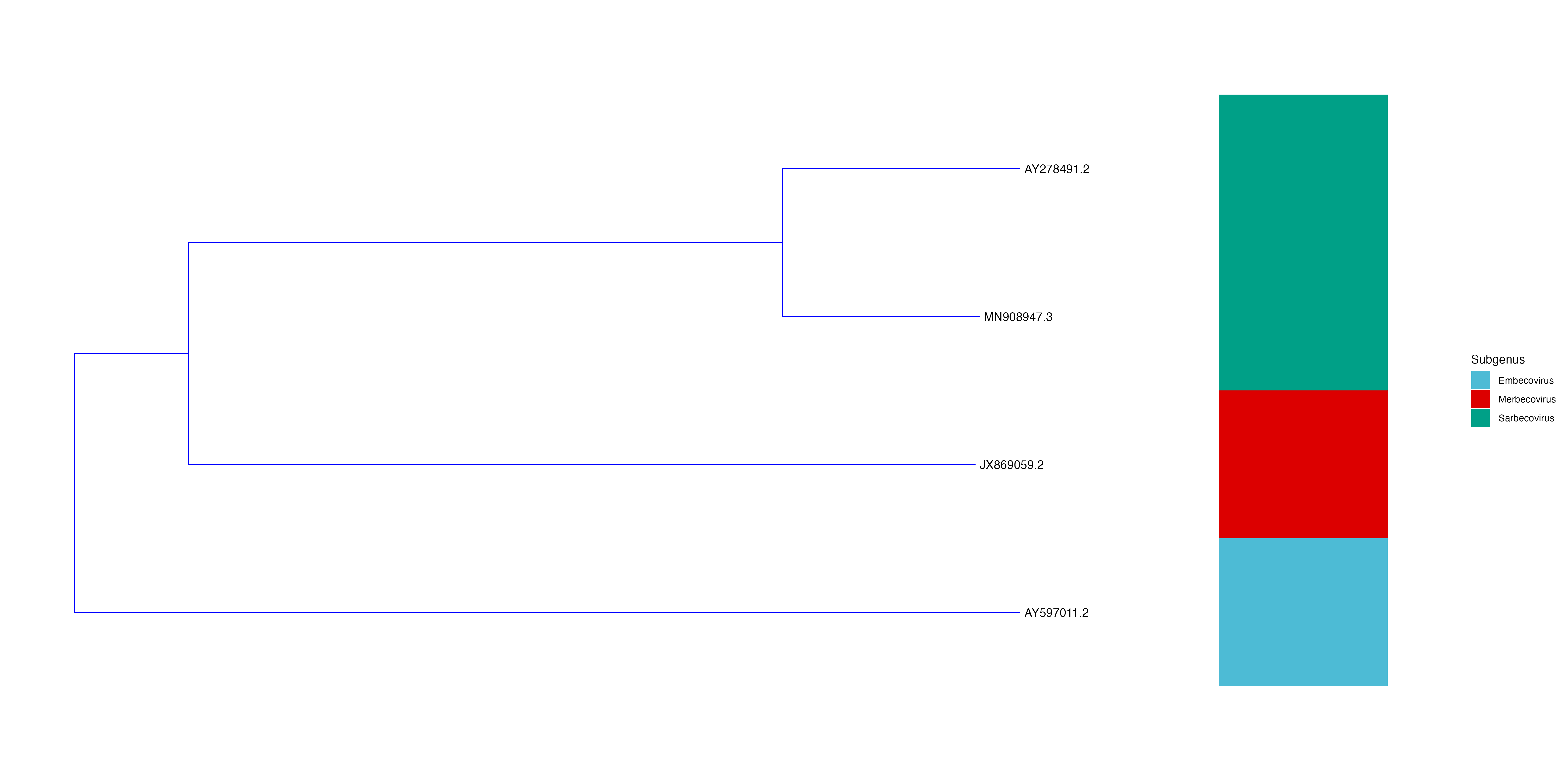
7. Now you can annotate the tree. In this example, the subgenus column is used.

    p3 <- p2 + new_scale_fill() + 
            geom_fruit(data = meta, 
                      geom = geom_tile, 
                      mapping = aes(y = ID, fill = Subgenus),
            offset = 0.3, pwidth = 0.1) +
            scale_fill_manual(
          values=c("#4DBBD5FF", "#DC0000FF", "#00A087FF"))
   

   Note: adjust the offset, pwidth and colours as defined in scale_fill_manual according personal taste

8. Plot and save

    plot(p3)
    ggsave("./lineage.png", p3, width = 20, height = 10)
   

   

back